PIC方法以及FDM方法

A polynomial Particle-in-cell method

related work

Finite difference method FDM

1. The initial velocity field is known and divergence free
2. Coordinates of a set of marker particles is known - showing which regions are fluid and which are not fluid
3. Pressure field is calculated so that the rate of change of the divergence of velocity is zero, which requires the solution of Poisson’s Equation - which can be done via an SOR method
4. Two components of acceleration are calculated
5. Marker particles move according to the velocity field
6. Adjustments are made for passage of marker particles across cell boundaries - i.e. the velocity changes when a cell is emptied and filled with fluid

The marker particles are not like the particle-in-cell method, i.e. the marker particles do not participate in the calculation, where as in the particle-in-cell method, they do.

Use the Conservative Form of the Navier-Stokes Equations:

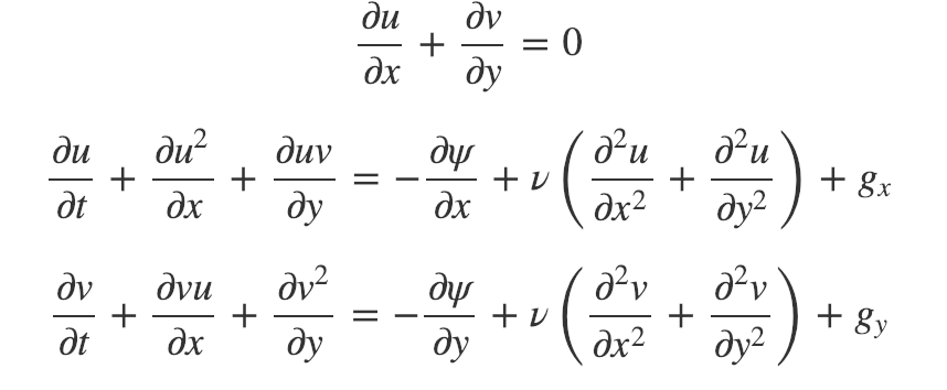
Harlow and Welch use ψψ to denote a pressure at a constant density i.e. $\frac{p}{p}$

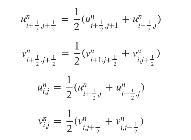
• Indices i and j count the centre of each cell
• Cell boundaries are labelled with half-integer values
• The superscript n+1 is used for time and where it is not used n is implied

The Finite Difference approximations are:

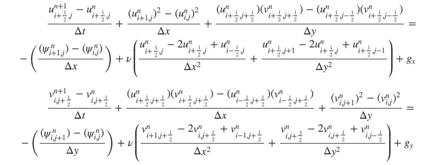
Some of the velocity values are not located at the centre of the mesh diagram, so an average of adjacent values is taken - i.e. the average of the velocity at the closest two points - which could be the vertical or horizontal direction, depending on which are the adjacent points

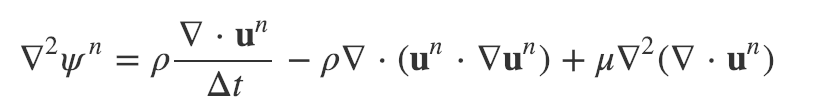
Harlow and Welch now take the divergence of the momentum equation:求散度

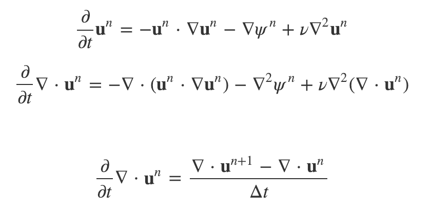Applying the principle of continuity:

• The divergence of velocity at the new timestep un+1=0un+1=0
• The divergence at the current timestep un≠0un≠0

Re-arrange for a form of the Poisson Equation at time n:

【欧几里得空间：这些数学空间可以被扩展来应用于任何有限维度，而这种空间叫做 n维欧几里得空间（甚至简称 {\displaystyle n} 维空间）或有限维实内积空间。

【拉帕拉斯算子

拉普拉斯算子是 n 维欧几里得空间中的一个二阶微分算子，其定义为对函数 先作梯度运算（)）后，再作散度运算(）的结果。因此如果 )是二阶可微的实函数，则 的拉普拉斯算子定义为：

二维空间

$\Delta f = \frac{\partial^2f}{\partial x^2} + \frac{\partial^2 f}{\partial y^2}$

三维空间$\Delta f = \frac{\partial^2 f}{\partial x^2} + \frac{\partial^2 f}{\partial y^2} + \frac{\partial^2 f}{\partial z^2}$

【泊松方程$\Delta\varphi=f$

${\nabla}^2 \varphi = f$

在三维直角坐标系，可以写成

】

Harlow and Welch say that you can neglect viscosity in the Poisson Equation with strict convergence critera

The loop in time is like this:

• Compute the RHS of the Poisson Equation at n
• Compute pressure using Poisson Equation at n
• Compute velocities at n+1 using Momentum Equations (from the pressure previously calculated at n)

The divergence of velocity must also vanish at the boundaries 散度

Marker Particles

Harlow and Welch developed (a now obsolete) particles method for tracking the motion of the free surface

They actually track the motion of particles throughout the fluid (not just at the free surface)

Linear interpolation is performed to calculate the velocity with which a particle should move

The interpolation weighting depends on the distance of the particle from the nearest velocity point

Boundary Conditions at Rigid Walls - Velocity

Rigid walls may be of two types:

No-slip

Free-slip (could be a plane of symmetry - or a greased surface)

• At the wall v=0v=0
• On the fluid side v≠0v≠0
• On the outside v′=−v (no slip)
• On the outside v′=+v (free slip)

(Similarly for horizontal walls)

In general:

• the tangential velocity reverses or remains unchanged for no-slip or free slip
• the normal velocity reverses for a free slip wall
• the normal velocity is calculated to ensure the divergence vanishes for an external cell for a no-slip wall

Boundary Conditions at Rigid Walls - Pressure¶

The boundary condition for ψ must be consistent with the velocity

Vertical wall From the momentum equation for uu (with the reversal of all normal velocities and no change in the tangential velocity):

ψ′=ψ±gxΔx

+⇒+⇒ fluid is on the left of the wall

−⇒−⇒ fluid is on the right of the wall

Horizontal wall From the momentum equation for vv:

ψ′=ψ±gyΔy

+⇒+⇒ fluid is below the wall

−⇒−⇒ fluid is above the wall

No slip wall

Condition is that the divergence of velocity on the outer cell must be zero:

Vertical wall

ψ′=ψ1±gxΔx±(2νu1Δx)ψ′=ψ1±gxΔx±(2νu1Δx)

+⇒+⇒ fluid is on the left of the wall

−⇒−⇒ fluid is on the right of the wall

Horizontal wall

ψ′=ψ1±gyΔy±(2νv1Δy)ψ′=ψ1±gyΔy±(2νv1Δy)

+⇒+⇒ fluid is on the left of the wall

−⇒−⇒ fluid is on the right of the wall

phase space

In dynamical system theory, a phase space is a space in which all possible states of a system are represented, with each possible state corresponding to one unique point in the phase space. For mechanical systems, the phase space usually consists of all possible values of position and momentum variables. The concept of phase space was developed in the late 19th century by Ludwig Boltzmann, Henri Poincaré, and Willard Gibbs.[1]

Particle-in-cell

the method amounts to following the trajectories of charged particles in self-consistent electromagnetic (or electrostatic) fields computed on a fixed mesh.

B样条

• curvature
• 学习 particle rendering